
Author
Last year our team had to analyze V8 bytecode. Back then, there were no tools in place to decompile such code and facilitate convenient navigation over it. We decided to try writing a processor module for the Ghidra framework. Thanks to the features of the language used to describe the output instructions, we obtained not only a readable set of instructions, but also a C-like decompiler. This article is a continuation of the series (1, 2) on our Ghidra plugin.
Several months went by between writing the processor module and this article. In this time, the SLEIGH specification remained unchanged, and the described module works on versions 9.1.2 – 9.2.2, which have been released during the last six months.
On ghidra.re and in the documentation distributed with Ghidra there is a fairly good description of the capabilities of the language. These materials are worth reading before writing your own modules. Preexisting processor modules by the framework’s developers might be excellent examples, especially if you know their architecture.
You can see in the documentation that the processor modules for Ghidra are written in SLEIGH, a language derived from the Specification Language for Encoding and Decoding (SLED), which was developed specifically for Ghidra. It translates machine code into p-code (the intermediate language that Ghidra uses to build decompiled code). As a language for describing processor instructions, it has a lot of limitations, although they can be reduced with the p-code injection mechanism implemented as Java code.
The source code of the new processor module is presented on github. This article will review the key concepts that are used in the development of the processor module using pure SLEIGH, with certain instructions as examples. Working with the constant pool, p-code injections, analyzer, and loader will be or have already been reviewed in other articles. Also you can read more about analyzers and loaders in The Ghidra Book: The Definitive Guide.
Where to begin
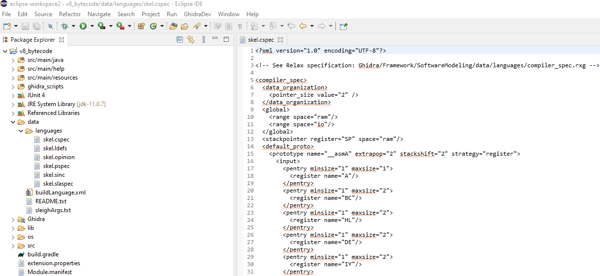
The work will require an installed Eclipse IDE, to which the plugins that come supplied with Ghidra (GhidraDev and GhidraSleighEditor) need to be added. Then the Ghidra Module Project with the name v8_bytecode is created. The new project contains template files that are important for the processor module; we will modify them to suit our needs.
For a general overview of the files we will need to work with, we can refer to the official documentation or the recently released The Ghidra Book: The Definitive Guide by Chris Eagle and Kara Nance. Here is a description of these files.
- *.сspec: compiler specification
- *.ldefs: the definition of the language. It contains the parameters of the processor module that are displayed in the interface. It also contains links to *.sla files, the processor specification, and the compiler spec.
- *.pspec: processor specifications
- *.opinion: loader configurations; given that we will be describing only one file type, the opinion file can be left blank; it will not be needed.
- *.slaspec, *.sinc: files that describe the registers, instructions, etc., for the processor in SLEIGH
After the first launch of your project, a file with the .sla extension will also appear. It is generated based on the SLASPEC file.
Before getting down to developing the processor module, you need to work out what registers there are, how to work with them, with the stack, etc., for the chosen processor or interpreter.
About V8 registers
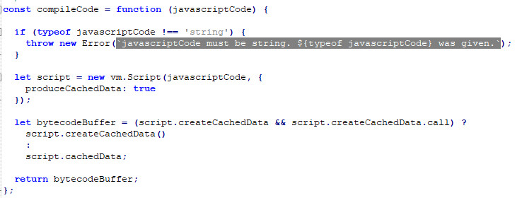
The JSC file that interests us was built using the JavaScript Node.js 8.16.0 runtime environment via bytenode (this module will either come supplied with Node.js or it will need to be installed via npm). In essence, bytenode uses the documented functionality of Node.js to create the compiled file. This is the source code of the function that compiles JSC files from JS:
You can download Node.js both in compiled form and as raw source files. Upon a detailed study of the source files and instruction examples, it becomes clear how the registers are encoded in bytecode (the file’s bytecode-register.cc and bytecode-register.h will be useful to understand the index computation). Examples of V8 instructions with register index computations in line with Node.js:
# 1e: Star instruction
# f9: r2, as 2 = -5 -(-7)
 1e f9             Star r2

# 1f: Mov instruction
# fb: r0, as 0 = -5 -(-5)
# f7: r4, as 4 = -5 -(-9)
 1f fb f7          Mov r0, r4

# 1d: Ldar instruction
# fe: <closure>,as -3 = -5 –(-2)
 1d fe             Ldar <closure>

# 11: LdaImmutableContextSlot instruction
# ff: <context>, as -4 = -5 –(-1)
# 1c: slot_index, uint
# 01: depth, uint
 11 ff 1c 01      LdaImmutableContextSlot <context>, [28], [1]

# 1f: Mov instruction
# 02: a0, as 0 = -5 –2 -(-7) + argCount -1 -1,  argCount=2
# f8: r3, as 3 = -5 -(-8)
 1f 02 f8          Mov a0, r3

# 1f: Mov instruction
# 02: a7, as 7 = -5 –2 -(-7) + argCount -1 -1,  argCount=9
# ed: r14, as 14 = -5 -(-19)
1f 02 ed          Mov a7, r14

# 1d: Ldar instruction
# : <this>, as 0 = -5 –3 -(-7) + argCount -1,  argCount=2
1d 03             Ldar <this>
If it seemed to you that the aX registers are encoded using different bytes, depending upon the number of function arguments, then you would be right. The following chart presents this more clearly.
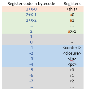
Here, X is the number of arguments of the current function ignoring the transmitted <this>; aX’s are the registers that contain the function arguments; rN’s are the registers used as local variables. The registers might be encoded with 1-byte values for regular instructions, 2-byte values for instructions marked Wide, and with 4-byte values for instructions marked ExtraWide. Sample encoding of a Wide instruction with explanations:
# 00: Wide instruction
# 2b: Add instruction (Add register to accumulator)
# ff da: r33: as 33 = -5 –(-38)
# 01 03: slot_index, uint
00 2b da ff 03 01 Add.Wide r33, [259]
Read more about Node.js and V8 in Sergey Fedonin’s article.
It is worth noting that SLEIGH is not totally suited for interpretable bytecodes of this kind, so the written processor module has certain limitations. For example, work is defined with no more than 124 rN registers and 125 aX registers. We attempted to resolve this problem using a stack-based communication model with registers, as it was more in line with the overall concept. However, in this instance, the disassembled bytecode was harder to read:
Also, without the introduction of additional pseudo-instructions, registers, or memory regions, it was impossible to compute the argument register name in accordance with Node.js, given that there was no information available on the number of arguments. In light of this, we decided to insert numbers in the function argument register names (X in aX) in reverse order. This does not hamper the parsing of the code, which was an important criterion for us. However, it might be confusing when comparing the results of a disassembled program’s instructions in different tools.
After studying what needs to be described, we can move on to composing the files we need for the processor module.
CSPEC
You can find some information on the tags used in CSPEC files in the framework source files on github. The file description states:
The compiler specification is a required part of
a Ghidra language module for supporting disassembly and analysis of a
particular processor. Its purpose is to encode information about a
target binary which is specific to the compiler that generated that binary. Within Ghidra, the SLEIGH specification allows the decoding of machine instructions for a particular processor, like Intel x86, but
more than one compiler can produce those instructions. For a particular target binary, understanding details about the specific compiler used to build it is important to the reverse engineering
process. The compiler specification fills this need, allowing concepts like parameter
passing conventions and stack mechanisms to be formally described…
It also becomes clear that the tags are used for the following purposes:
- Compiler specific p-code interpretation
- Compiler datatype organization (we used <data_organization>)
- Compiler scoping and memory access (we used <global>)
- Compiler special purpose registers (we used <stackpointer>)
- Parameter passing (we used <default_proto>)
When studying the template structure, the described tags in the documentation, and examples of similar files, we can try to compile a file to suit our needs.
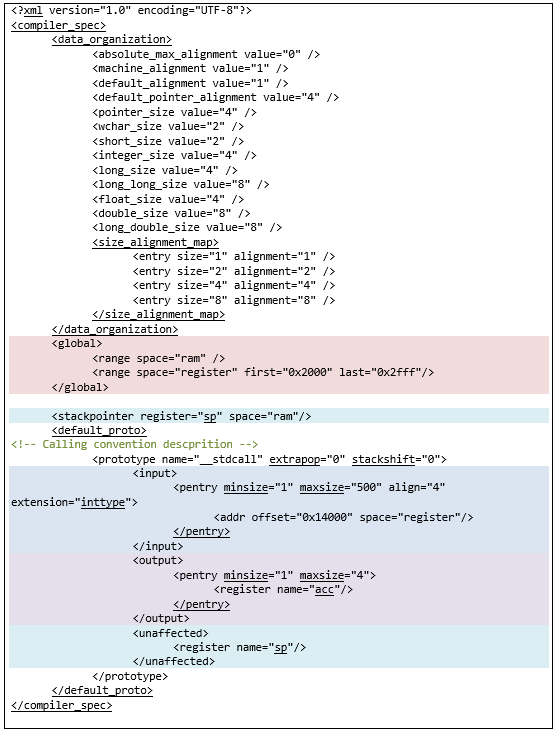
The <data_organization> and <stackpointer> tags are fairly typical; let’s take a closer look at the tag <prototype> in <default_proto>, which partially describes the agreement on function calling. For this, we define the following: <input>, <output>, <unaffected>.
As mentioned above, arguments are passed to the function through the aX registers. In a module, registers must be defined as a contiguous sequence of bytes at offset in some space. As a rule, in such cases, a specially designated space named register is used. However, in theory, there is nothing to stop you from using any other space. When there are a large number of registers performing more or less the same functions, it is simplest not to denote each of them separately, rather you can simply specify the offset with a set of registers in a space and use that to define them. Therefore, we mark the memory region in the register space (space="register") in the <input> tag for registers through which the arguments are passed into functions, at offset 0x14000 (0x14000 is not set in stone; this is just an offset at which the aX registers will be defined in *.slaspec below).
By default, the result of the function call is saved in the accumulator (acc), which needs to be denoted in the <output> tag. For alternative register variations, where the values returned by the functions are stored, we can define the logic when describing instructions. In the <unaffected> tag, we note that the function calls have no impact on the register that stores the stack pointer.
To work with some registers, the most convenient option would be to define them as globally changeable. So in the <global> tag, we define the range of registers in the register space at offset 0x2000.
LDEFS
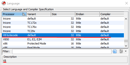
Moving on to the language definition: this is a file with the .ldefs extension. It requires a little information for describing: the byte order (we have le), names of key files (* .sla, * .pspec, and *.cspec), id, and bytecode name, which will be displayed in the list of supported processor modules when importing a file into Ghidra. If we ever need to add a processor module for a file compiled by a version of Node.js that is significantly different from the current one, then we describe it there by creating another tag, as it is done to describe processor families in * .ldefs modules supplied as part of Ghidra.
<?xml version="1.0" encoding="UTF-8"?>

<language_definitions>
  <language processor="V8 bytecode"
            endian="little"
            size="32"
            variant="default"
            version="1.0"
            slafile="skel.sla"
            processorspec="skel.pspec"
            id="V8:LE:32:default">
    <description>V8</description>
    <compiler name="default" spec="skel.cspec" id="default"/>
  </language>
</language_definitions>
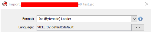
The practical application of information that does not relate to the definition of the files will be visible when attempting to import the file.
PSPEC
The situation with the processor specification (file with the .pspec extension) is more complicated in terms of documentation. In this case, you can turn to ready-made solutions within the framework itself or to the processor_spec.rxg file (we have not looked at an option with a full-scale parsing of Ghidra source codes). At the time when the module was written, there was nothing more detailed available. In time, the developers will probably publish official documentation.
In this current project, the only thing we might need from the processor specification at the moment is a program counter; we’ll leave this tag from the standard template of the newly built project (we could in fact leave <processor_spec> empty).
<?xml version="1.0" encoding="UTF-8"?>

<processor_spec>
  <programcounter register="pc"/>
</processor_spec>
SLASPEC
Now we can get on with the actual description of the instructions in SLEIGH in a file with the .slaspec extension.
Basic definitions and macros of the preprocessor
When describing it, firstly, we need to specify the byte order. We can also define alignment and constants which might be needed in the description process, by using preprocessor macros.
define endian=little;
define alignment=1;

# $(SIZE) will be equal to 4
@define SIZE "4"
@define RECV_ARG	"1"
@define PROPERTYTYPE 	"3"
The address spaces that we will need to describe the bytecode (we created spaces with the names register and ram) shall be defined by way of define space, while the registers, by way of define register. The offset value in the definition of the registers is not of fundamental importance; what is most important is that they are located on different offsets. The number of bytes that is taken up by the registers is defined by the size parameter. Remember that the information defined here must correspond to calls to similar abstractions and values within *.cspec and the analyzer, if you refer to these registers.
# define space spacename attributes

# type=(ram_space|rom_space|register_space)
# size=integer
# default – use this space unless another one was specified
# wordsize=integer

# ram definition
define space ram type=ram_space size=$(SIZE) wordsize=1 default;
# register space definition
define space register type=register_space size=$(SIZE);
# offset can be important for analyzer purposes, you don`t define different registers in the same address ranges at the same space

# function argument registers, mentioned in <input> tag in cspec
define register offset=0x14000 size=4
[
	a0 a1 a2 a3 a4 a5 a6 a7 a8 a9 a10 a11 a12 a13 a14 a15 a16
	a17 a18 a19 a20 a21 a22 a23 a24 a25 a26 a27 a28 a29 a30 a31 a32
	a33 a34 a35 a36 a37 a38 a39 a40 a41 a42 a43 a44 a45 a46 a47 a48
	a49 a50 a51 a52 a53 a54 a55 a56 a57 a58 a59 a60 a61 a62 a63 a64
	a65 a66 a67 a68 a69 a70 a71 a72 a73 a74 a75 a76 a77 a78 a79 a80
	a81 a82 a83 a84 a85 a86 a87 a88 a89 a90 a91 a92 a93 a94 a95 a96
	a97 a98 a99 a100 a101 a102 a103 a104 a105 a106 a107 a108 a109 a110 a111 a112
	a113 a114 a115 a116 a117 a118 a119 a120 a121 a122 a123 a124 a125
];
define register offset=0x3000 size=4
[
	r0 r1 r2 r3 r4 r5 r6 r7 r8 r9 r10 r11 r12 r13 r14 r15 r16
	r17 r18 r19 r20 r21 r22 r23 r24 r25 r26 r27 r28 r29 r30 r31 r32
	r33 r34 r35 r36 r37 r38 r39 r40 r41 r42 r43 r44 r45 r46 r47 r48
	r49 r50 r51 r52 r53 r54 r55 r56 r57 r58 r59 r60 r61 r62 r63 r64
	r65 r66 r67 r68 r69 r70 r71 r72 r73 r74 r75 r76 r77 r78 r79 r80
	r81 r82 r83 r84 r85 r86 r87 r88 r89 r90 r91 r92 r93 r94 r95 r96
	r97 r98 r99 r100 r101 r102 r103 r104 r105 r106 r107 r108 r109 r110 r111 r112
	r113 r114 r115 r116 r117 r118 r119 r120 r121 r122 r123
];

define register offset=0x0080 size=$(SIZE) [ range_size acc sp];
# 0x2000- 0x2fff was mentioned in <global> tag in cspec
define register offset=0x2000 size=$(SIZE) [ pc fp _context _closure ];
define register offset=0x2020 size=$(SIZE) [ True False Undefined TheHole Null JSReceiver ];
Description of instructions
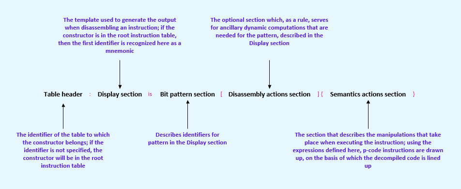
We read in the documentation that the instructions are defined through tables that consist of one and more constructors, and which have family symbol identifiers associated with them. Tables in SLEIGH are what helped to create family symbols. We won’t go into great detail on definitions of symbols in this article; you’d be better off reading Introduction to Symbols, but probably the concept will be clear after reading this article. The constructors consist of five parts:
- Table header
- Display section
- Bit pattern section
- Disassembly actions section
- Semantics actions section
It might look scary for now, so we’ll describe the main idea.
- The table header either contains the identifier, which can be used in other constructors, or is blank (in which case there is the description of the instruction).
- The display section is a template for how to display the instruction into the Ghidra listing.
- The bit pattern section is a list of identifiers that take the real bits of the program for instructions and are displayed in the listing according to the pattern of the display section (sometimes using the next section).
- The disassembly actions section supplements the bit pattern section with its computations if it is insufficient in its pure form.
- The semantics actions section describes what an instruction does, so as to show this in the decompiler.
Initially, there is a root instruction table (the identifier instruction is attached to it), all the described constructors with an empty table header become a part of it, and the first identifier of these constructors in the display section is recognized as a mnemonic of the instructions.
For constructors with an identifier in the table header, a new table with the appropriate name is created. If it already exists, the constructor becomes a part of that same table. This case will be covered in the section on the range of registers. When using the identifier of a table in another table, the referenced table is treated as a part to the current one. In other words, the creation of a table whose identifiers aren’t used anywhere (they will be wholly unconnected with the root table of instructions) has no practical point.
Here are a few documented features of the Display section, which will be needed as we move on:
- The caret (^) separates identifiers and/or characters in section between which there should be no spaces.
- The quotation marks (“”) are used to insert hard-coded strings that will not be considered an identifier.
- Whitespace characters are truncated at the beginning and end of the section, and the sequence of these characters is compressed into a single space.
- Some punctuation marks and special characters are inserted into the template (not used for any specific functions, unlike, for example, hashes (#), which are used for comments).

Tokens and their fields
Bit fields need to be defined to describe the instruction constructors. Through them, the bits of the program become tied to certain abstractions of the language into which the translation will take place. For example, mnemonics or operands can be such abstractions. The fields are defined during token definition; the syntax of their definition is as follows:
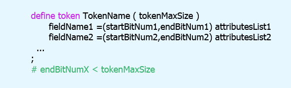
The size of the token (tokenMaxSize) must be a multiple of 8. This might be inconvenient if the operands or nuances for the instruction are coded using a smaller number of bits. On the other hand, this is compensated by the ability to create fields of different sizes, positionally decoding any bits within the size specified by the token. The following conditions must be observed for such fields: startBitNumX and endBitNumX are in the range from 0 to tokenMaxSize-1 inclusive and startBitNumX <= endBitNumX.
There was no need to create fields that differed in size from the token for the parsed V8 bytecode. However, if there were such fields, and if they were used together, they would be unified by way of logic operators “&” or “|.”
Note: even if you use a field or a combination of fields in the bit pattern section that do not cover the full size of the token to which they belong with their bitmasks, the number of bits determined by the token size will still be taken from the program bytes for the operand.
Now let’s describe a really simple bytecode instruction that does not have operands. We define the field that will describe the instruction opcode. As we see above in the section about V8, the instruction code is described by one byte (there are also Wide and ExtraWide instructions, but they won’t be considered here as, in essence, they simply use operands of large sizes along with additional byte for the instruction opcode). Thus we get:
# 8 – token size
# field op includes bits 0 to 7
define token opcode(8)
	op = (0,7)
;
Now, using the op field to identify the first and only opcode that defines the Illegal and Nop instructions, we write the constructors for them:
# “op=0xa7” is a constraint dictating to interpret a byte as an instruction Illegal
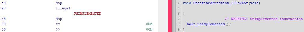
:Illegal is op = 0xa7 unimpl # decompilation will be interrupted
# was not presented in our version, only for switch purposes
:Nop is op = 0xa8 {} # empty decompiled code
Byte 0xa7 in the Ghidra listing will be displayed as an Illegal instruction that has no operands. In the example for this instruction, the unimpl keyword was used. This is an unimplemented command, and further decompiling will be interrupted, which is convenient for tracking unimplemented semantic descriptions. An empty semantic section is left for Nop, meaning that the command will not affect the display in the decompiler, which is what this instruction should do. In actual fact, Nop does not exist as an instruction in our version of Node.js; we introduced it artificially to implement the functionality of SwitchOnSmiNoFeedback, but this will be covered in Vladimir Kononovich’s article.
Describing operands and semantics
Let’s complicate the concept: we’ll describe a constructor for the LdaSmi operation in which an integer is loaded into the accumulator (acc in the definition of the register space), and for the AddSmi operation, which essentially is the addition of the value in the accumulator to an integer.
For current and future needs, we’ll define a few more fields after the manner of operands in bytecodes.h of Node.js, and we will create them in a new token named “operand,” as these fields will have a different purpose than “op”. Creating several fields with identical bitmasks might be to facilitate perception and to use several fields of one token within one instruction (see the example with AddSmi).
define token operand(8)
	kImm = (0,7) signed dec
	kIdx = (0,7)
	kIdx_2 = (0,7)
	kUImm = (0,7)
	kFlag8 = (0,7)
	kIntrinsicId = (0,7)
	kReg = (0,7)

;
From the point of view of the listing, we’d like to see something like LdaSmi [-0х2]. Therefore, we define a mnemonic in the display section and then we write the field names in the template, which should be taken from the disassembly actions section or the bit pattern section (the square brackets are not obligatory here; they’re just for appearance).
For the AddSmi instruction, in the bit pattern section, in addition to the op field that sets the limit on the opcode, the fields appear from the operand token, divided by a semicolon (;). They will be placed in the display section as operands. Real bits are mapped in the order in which the fields are specified in the bit pattern section. We implement the instruction logic in the semantics actions section, using the documented operations; this is what an interpreter would do when fulfilling these instructions.
#  LdaSmi <imm>
#  Load an integer literal into the accumulator as a Smi.
:LdaSmi [kImm] is op = 0x3; kImm {
  acc = kImm;
}
#  AddSmi <imm>
#  Adds an immediate value <imm> to the value in the accumulator.
#   kIdx is needed for optimization purposes
:AddSmi [kImm], [kIdx] is op = 0x36; kImm; kIdx {
  acc = acc + kImm;
}
There can also be, for example, registers, context variables (more on them later), and combinations of the fields of one token or fields with context variables, divided by a semicolon (;).
This is what the listing window looks like with the described instructions with the PCode field enabled in the Edit the Listing fields menu of the Ghidra listing. The decompiler window will not yet be indicative due to code optimization, so, at this stage, it is worth focusing only on the intermediate p-code operations.


In V8 bytecode, all instructions whose mnemonics start with lda imply loading a value into the accumulator. However, if you want to clearly see the acc register in the bytecode instructions, you can define it for display in the constructor. In this case, it makes no difference in which position in the bit pattern section the acc is located, since it is not a field and does not occupy instruction bits, although it does need to be written in.
:LdaSmi acc, [kImm] is op = 0x3; kImm; acc {
	acc = kImm;
}

The instructions for returning values from the function are implemented using the return keyword and, as already mentioned, the value is returned most often through the accumulator, when calling the function:
:Return is op = 0x95 {
	return [acc];
}
Outputting registers over bitmasks
The instructions we have described above do not use registers as operands. Now, though, we implement the constructor of the Mul instruction, under which the accumulator is multiplied by the value that is stored in the register.
In the Basic Definitions and Macros of the Preprocessor code section, the registers were already declared, but in order for the necessary registers to be selected depending upon the bits presented in the bytecode, we need to bind their list to the corresponding bitmasks. The kReg field is 8 bits in size. Using the attach variables construction, we sequentially define to which bitmasks, from 0b to 11111111b, the aforementioned registers will correspond as part of the subsequent use of fields from the set list (only kReg in our case) in the constructors. For example, it is evident in this description that the operand coded as 0xfb (11111011b) is interpreted as the r0 register when it is described through kReg.
# attach variables [ fields ] [ registers ]
attach variables [ kReg ] [
	_ _ a0 a1 a2 a3 a4 a5 a6 a7 a8 a9 a10 a11 a12 a13 a14 a15 a16
	a17 a18 a19 a20 a21 a22 a23 a24 a25 a26 a27 a28 a29 a30 a31 a32
	a33 a34 a35 a36 a37 a38 a39 a40 a41 a42 a43 a44 a45 a46 a47 a48
	a49 a50 a51 a52 a53 a54 a55 a56 a57 a58 a59 a60 a61 a62 a63 a64
	a65 a66 a67 a68 a69 a70 a71 a72 a73 a74 a75 a76 a77 a78 a79 a80
	a81 a82 a83 a84 a85 a86 a87 a88 a89 a90 a91 a92 a93 a94 a95 a96
	a97 a98 a99 a100 a101 a102 a103 a104 a105 a106 a107 a108 a109 a110 a111 a112
	a113 a114 a115 a116 a117 a118 a119 a120 a121 a122 a123 a124 a125
	r123 r122 r121 r120 r119 r118 r117 r116 r115 r114
	r113 r112 r111 r110 r109 r108 r107 r106 r105 r104 r103 r102 r101 r100 r99 r98
	r97 r96 r95 r94 r93 r92 r91 r90 r89 r88 r87 r86 r85 r84 r83 r82
	r81 r80 r79 r78 r77 r76 r75 r74 r73 r72 r71 r70 r69 r68 r67 r66
	r65 r64 r63 r62 r61 r60 r59 r58 r57 r56 r55 r54 r53 r52 r51 r50
	r49 r48 r47 r46 r45 r44 r43 r42 r41 r40 r39 r38 r37 r36 r35 r34
	r33 r32 r31 r30 r29 r28 r27 r26 r25 r24 r23 r22 r21 r20 r19 r18
	r17 r16 r15 r14 r13 r12 r11 r10 r9 r8 r7 r6 r5 r4 r3 r2 r1 r0 pc fp _closure _context
];
Now, when registers are attached to the kReg variable, this variable can be used in the constructors:
#  Mul <src>
#  Multiply accumulator by register <src>.
#   kIdx is needed for optimization purposes
:Mul kReg, [kIdx] is op = 0x2d; kReg; kIdx {
	acc = acc * kReg;
}

We can make the construction more complex to make the constructor correspond with higher-level descriptions of instructions from the interpreter-generator.cc Node.js source files. We move the kReg field to a separate constructor, the table identifier of which, located in the table header section, we’ll name src. In its semantics actions section appears a new keyword — export. Not going into great detail about the construct of p-code, essentially export implies the definition of the value that must be placed in the semantics actions section of the constructor in place of src. The output to Ghidra doesn’t change.
src: kReg is kReg {  # src – table identifier
    export kReg;     # dynamic export for manipulation in semantic section where this constructor will be used
}

#  Mul <src>

#  Multiply accumulator by register <src>.
:Mul src, [kIdx] is op = 0x2d; src; kIdx {
	acc = acc * src;
}
Examples of instructions, similar in terms of description, which will be needed later for testing the module on a real file:
dst: kReg is kReg {export kReg;}

:Ldar src is op = 0x1d; src {
	acc = src;
}
:Star dst is op = 0x1e; dst {
	dst = acc;
}
Jumping to addresses with goto
We encounter conditional and unconditional transitions in the bytecode via relative offsets from the current address. To jump to an address or label in SLEIGH, we use the goto keyword. It is noteworthy for the definition that the bit pattern section uses the kUImm field, although it is not used in its pure form. The value calculated in the disassembly actions section is exported to the display section through the rel identifier. inst_start is a predefined symbol for SLEIGH and contains the address of the current instruction.
# inst_start – address of current instruction
# * - dereference operator
# Jump <imm>
# Jump by the number of bytes represented by the immediate operand |imm|.
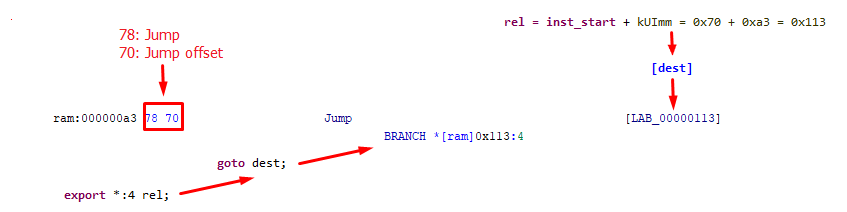
:Jump [rel] is op = 0x78; kUImm [ rel = inst_start + kUImm; ] {
# rel:4 for resolving variable size
goto [rel:4];
}
SLEIGH compiles successfully. That said, in this variation (see the following listing), judging by the output, no varnodes can be created (these are objects that are manipulated by the p-code instruction) that contain a binding to a specific space.

We use the method recommended by the developers and take out part of the definition by creating an additional constructor with the dest identifier. The *[ram]:4 rel construction does not mean we take 4 bytes over the rel address. In fact, the rel address is exported in the ram space. The asterisk (*) operator in SLEIGH means dereferencing, but in this specific instance, it relates to the nuance of creating a varnode (there is more about this in Dynamic references).
Specifying the [ram] space can be omitted (there’s an example in the comments), because during the definition, we specified it as the default space. As we can see in the p-code instructions, the offset was marked as belonging to ram.
# calculate destination for jumps

# * - dereference operator
# inst_start – address of current instruction

dest: rel is kUImm [ rel = inst_start + kUImm; ] {
#  export *:4 rel;
  export *[ram]:4 rel;
}
# Jump <imm>
# Jump by the number of bytes represented by the immediate operand |imm|.
:Jump [dest] is op = 0x78; dest {
	goto dest;
}
The JumpIfFalse instruction appears a little more complicated due to the use of the conditional construction. It is used in SLEIGH together with the goto keyword. For a greater conformity to JS concepts, the False value was previously defined as a register, and we note that, in *.pspec, the register space range to which it is attached is marked as global. Thanks to this, it is displayed in the pseudocode in accordance with the register name and not with the numerical value.
#  JumpIfFalse <imm>
#  Jump by the number of bytes represented by an immediate operand if the
#  accumulator contains false.
:JumpIfFalse [dest] is op = 0x86; dest {
	if (acc == False) goto dest;
}

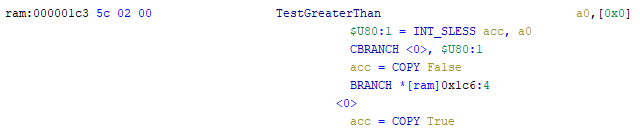
In the examples provided, the transition is made to the address calculated relative to inst_start. Let’s consider the TestGreaterThan instruction, which uses goto to jump to the label (<true> in the example below) and inst_next. As such, the jumpto the label should be intuitively clear: if the condition is true, then the instructions that come after the label`s position shall be fulfilled. The label is valid only within its semantics actions section.
The goto inst_next construction actually ends processing of the current instruction and transfers control to the next one. Note that “s>” is used to perform signed comparison (see the documentation).
#  TestGreaterThan <src>
#  Test if the value in the <src> register is greater than the accumulator.
#  kIdx is needed for optimization purposes
:TestGreaterThan src, [kIdx] is op = 0x5c; src; kIdx {
	if (src s> acc) goto <true>;
	acc =False;
	goto inst_next;
	<true>
	acc=True;
}
Several register operands
Previous instructions used no more than one register as an operand. Therefore, we’ll talk first about using more registers for this purpose.
The description of operands through identical constructors with different table identifiers (see constructors in the following example) can be of practical use within one single constructor of another table. We will apply such an option not only in terms of conformity to the description of the V8 instructions but also to avoid possible errors. For example, four operands of the CallProperty2 instruction are registers, identically specified in terms of the bitmask. The attempt to define the constructor as CallProperty2 kReg, kReg, kReg, kReg, [kIdx] generates an error in the SLEIGH compiler during an attempt to open the file using the processor module. Therefore, our module used constructors to create something similar to aliases:
callable: kReg is kReg {export kReg;}
receiver: kReg is kReg {export kReg;}
arg1: kReg is kReg {export kReg;}
arg2: kReg is kReg {export kReg;}
It is worth noting, of course, that it was also possible to solve this problem without defining new constructors. For example, by defining and registering the callable, receiver, arg1, and arg2 fields within a token and subsequently binding them to the list of registers using the attach command:
define token func(8)
  callable = (0,7)
  receiver = (0,7)
  arg1 = (0,7)
  arg2 = (0,7)
;
#  “…” is here to skip a definition similar to the previous one
attach variables [ callable receiver arg1 arg2] [_ _ a0 a1 … r0 pc fp _closure _context];
Each of these fields would work in a similar way to kReg in the previous examples. Which specific method to use is a matter of aesthetics.
Function calls
Also noteworthy in the CallProperty2 instruction is that in the semantics actions section, it uses the call [callable] construction, which we have not used prior to this. In V8, the function arguments are stored in the aX registers (as we noted in CSPEC). However, in terms of bytecode, we do not place arguments there immediately prior to calling the function (we can view cases when this does take place in the *.sinc file, such as for x86). The interpreter does this independently, as it has all the necessary information to do this itself. However, Ghidra does not have it, so in the semantics actions section we will manually write the arguments into registers. That said, we will need to restore the values of the involved registers after the call, since in the calling function, these registers can also store some values that are necessary to the code flow. You can save them through local variables:
callable: kReg is kReg {export kReg;}
receiver: kReg is kReg {export kReg;}
arg1: kReg is kReg {export kReg;}
arg2: kReg is kReg {export kReg;}

# Call <callable> <receiver> <arg_count> <feedback_slot_id>
# Call a JSfunction or Callable in |callable| with the |receiver| and
# |arg_count| arguments in subsequent registers. Collect type feedback
# into |feedback_slot_id|

:CallProperty2 callable, receiver, arg1, arg2, [kIdx] is op = 0x4d; callable; receiver; arg1; arg2; kIdx {
    # you can define locals as:
	local tmpArg1 = a0;
    # or “local tmpArg1:4 = a0;”
    # or in such manner:
	tmpArg2:4 = a1;
	a1 = arg1;
	a0 = arg2;
	call [callable];
	receiver = acc;
	a0 = tmpArg1;
	a1 = tmpArg2;
}
We can also save arguments in memory (in this case on the stack: sp is not used by instructions so it doesn’t affect the decompiler display) when using macros in the CallUndefinedReceiver1 example:
macro push(x){
	sp = sp - $(SIZE);
	*:$(SIZE) sp = x;
}
macro pop(x){
	x = *:$(SIZE) sp;
	sp = sp + $(SIZE);
}
:CallUndefinedReceiver1 callable, arg1, [kIdx] is op = 0x50; callable; arg1; kIdx {
	push(a0);
	a0 = arg1;
	call [callable];
	pop(a0);
}
When writing similar modules together with the loader and the analyzer, it is worth making sure that the order of the passed arguments coincides with the order of the function arguments, which are defined in the Java code part. It is also worth noting that it is important here to save no more function arguments than there are in the calling function, but this is difficult to implement in SLEIGH. A solution to the problem can be read in the article by Vyacheslav Moskvin about the injection of p-code instructions.
User-defined operations
In order not to lose instructions during decompilation, in which it is not planned or it is not possible to describe the semantics actions section, you can use user-defined operations. It is noteworthy that in the case of the acc, you do not need to specify the size explicitly since the register size is defined explicitly, . However, when passing, for example, numeric constants to such user operations, you have to explicitly specify the size of the passed value (as in the case with CallVariadicCallOther in the About the Register Ranges section later in the text). User-defined operations are defined as define pcodeop OperationName and are used in the semantics actions section of the constructors in a format similar to function calls in many programming languages.
define pcodeop TypeOf;
define pcodeop StackCheck;
define pcodeop GetGlobal;

:TypeOf is op = 0x45 {
	acc = TypeOf(acc);
}
:StackCheck is op = 0x91 {
	StackCheck();
}
:LdaGlobal [kIdx], [kIdx_2] is op = 0xa; kIdx; kIdx_2 {
#     it will be discussed in next paper, now let`s work without resolving constants
#	cp:4 = cpool(0,inst_start, kIdx, $(CP_CONSTANTS));
#     temp expression:
	cp:4 = kIdx;
	acc = GetGlobal(cp);
}
These operations might be used to inject p-code instructions in the analyzer: the call is added via the callotherfixup tag to the CSPEC file and the logic is denoted in the analyzer.
Without redefinition in Java code, user operations in the decompiler appear just as they were defined in the semantics actions section:

Testing the module
At this stage, we can already attempt to check the work of the processor module in practice. We compile the JSC file through bytenode from a small example in JS:
function func(n) {
	if (n > 1) {
		alert(n*n+12);
		return 1;
	} else{
		return -1;
	}
}
We’ll try to launch the project written based on this article and import the obtained JSC file into Ghidra. If something has been written incorrectly, Ghidra will display an error, and the number of the string causing the error will be located in the eclipse logs. When correcting the code, there is no need to rebuild the project: SLEIGH will be recompiled at the next attempt to open the file.
Just in case here is the archive with the files that we should have got. You can also view the full version of the tool written for the project in our company`s repository.
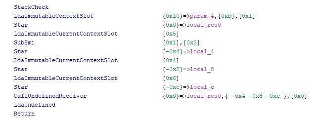
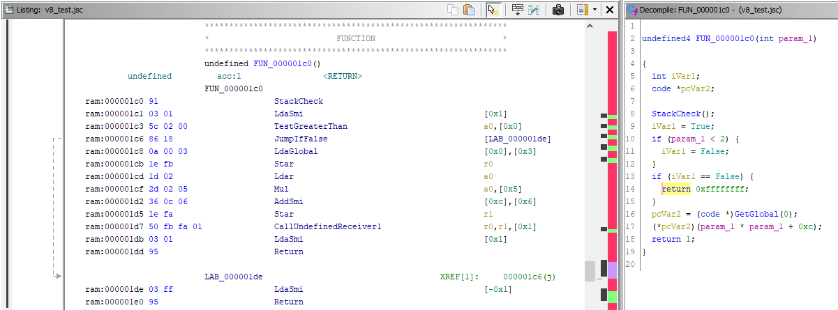
As we have described the instructions only, the file will not be analyzed and parsed into functions. The code is at offset 0x1c0. Press D there to convert bytes to instructions for that offset and F to create a function. This is how it will look:
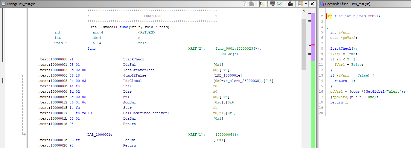
The output becomes clearer when we use other tools (in addition to SLEIGH) which are available to the module developers. For example, when work is added with the pool constant (the cpool keyword has been reserved to refer to it in SLEIGH), the opportunity arises to resolve the numeric identifier in the LdaGlobal command. This is what the function looks like in the latest version of our project (for comparison):
Of course, it would be nicer to see a better match to the source code written in JavaScript, but this cannot be achieved by describing instructions only in .slaspec (and .sinc) files. The next article in line gives a little more scope to imagination; it describes a mechanism for the injection of p-code operations allowing, with full access to all application resources, the manipulation of the instructions from which the p-code tree is created. It is on the basis of the created p-code tree that the decompilation result is drawn up and displayed in the interface.
About the register ranges
A number of instructions work with ranges, pairs, and triples of registers in V8 bytecode. From the point of view of encoding ranges, there is the code of the first register and the number of registers used in the range. For pairs and triples, only the initial register is specified, since the interpreter knows in advance how many registers to use for a given instruction.
# range
# 4a: CallProperty instruction
# f7: r4, as 4 = -5 -(-9)
# f6 07: r5-r11, as 5 = -5 -(-10) and there are 7 registers to pass
# 1a: for optimization purposes
@  173 : 4a f7 f6 07 1a    CallProperty r4, r5-r11, [26]

# pair
# 8f: ForInNext instruction
# f6: r5, as 5 = -5 -(-10)
# f2: r9, as 9 = -5 -(-14)
# f5: r6-r7, as 6 = -5 -(-11) and there are 2 registers to pass
# b9: for optimization purposes
@  758 : 8f f6 f2 f5 b9    ForInNext r5, r9, r6-r7, [185]

# triple
# 8d: ForInPrepare instruction
# f2: r9, as 9 = -5 -(-14)
# f1: r10-r12, as 10 = -5 -(-15) and there are 3 registers to pass
@   71 : 8d f2 f1          ForInPrepare r9, r10-r12
Based on the description, it is clear that a fairly simple solution would be to display the first register and their quantity when parsing instructions, meaning something like this: ForInPrepare r9, r10!3. A slightly bigger compromise for the sake of readability would be to output the first and last registers of the range, but, looking ahead, we could say that, as far as implementation is concerned, this would already require the use of tables consisting of several constructors.
Tables containing several constructors
As part of the project and for ease of perception, a decision was made to display the entire list of passed registers. There is no ready-made template to output register ranges in the display section. We can, though, be guided by principles that are similar to those used for the ARM processor module: the output of variables through a chain of constructors (only the principle itself; the implementation doesn’t suit us because of the difference in architectures).
Here you can clearly see the very case when a table with a certain identifier consists of several constructors. In essence, these are several constructors with the same identifiers in the table header section with different conditions in the bit pattern section. Looking at this description, you can realize that you have already implemented a similar table, describing the instructions — they are in the root instruction table and are selected depending on the opcode condition.
When working with an identifier in other constructors, the most suitable option will be selected. For example, if a constructor of a table is described with a certain condition and the next constructor doesn’t have one then if the first condition is true, the first option will be selected, regardless of the second one, even though the second does not formally contradict the condition, since it does not impose any conditions at all.
As we might assume, looking at the byte-by-byte description of the CallProperty instruction above, to display the entire range, we need to output the registers, starting from the first entry, focusing on the known first range register and the number of elements in it. In terms of the display section, the range is created from two constructors: rangeSrc and rangeDst. rangeSrc is a kind of initialisation, where we save the input data, while rangeDst will output the registers based on the information received. For rangeDst specifically, we need to create tables that consist of several constructors: at least to display ranges on the aX and rX registers separately.
To implement the conditions, a number of restrictions must be taken into account. It is recommended to check the values in the bit pattern section only using an equals sign (=) and you cannot directly clarify the value of the register or assign it a value in the disassembly actions section. This means we cannot use a temporary register. The start register and the length of the range might be different values, while the range, as previously mentioned, can be implemented both as aX registers and as rX registers; it can also have a zero length. It is already clear at this stage that if we don’t want to create an enormous amount of definitions for every occasion, it would be a good idea to have some counters, to ascertain how many registers we should output, and from which position.
Context variables
Context variables are suitable for resolving tasks. Their definition is similar to the definition of token fields. However, instead of real program bits, the fields in this case use bits of the specified register (contextreg below).
When writing through the fields defined in the register over the same bit ranges, the values will be overwritten (in some cases, compilation will not work), since these are bits of the same register. Our context variables, counter and offStart, use different bit ranges within the register, since in their meaning, they are different values.
It is important to note that the context variables must be declared before the constructors.
# context register for ranges
define register offset=0x00 size=8   contextreg;
define context contextreg
	# counter for range registers enumerating
      counter = (0,7)
	# variable to store the first register
      offStart = (8,16) signed
;
The documentation explains that context variables are usually used in the bit pattern section to check for the presence of some kind of context and are changed in the disassembly actions section. Therefore, in the constructor with the table identifier rangeSrc, which we will use to display the ranges, in the disassembly actions section, we save the code of the first range register into the context variable offStart, while the quantity goes into the context variable counter. We label the start of the range in the display section with an opening curly bracket ({).
It is also noteworthy that V8 doesn’t use the range_size register: it is introduced artificially to save the range size, thus making it more convenient to work with this value as part of the semantics actions section of the instruction constructor if necessary. It is rangeSrc that supplies the start register and the range size for the semantics actions section of the instruction.
rangeSrc: {  is kReg; kUImm  [ offStart = kReg; counter =  kUImm; ] { range_size = kUImm;  export kReg;}
# and it`s not difficult to modify range into pair and triple, you should just hardcode counter to 2 or 3 in rangeSrc
As part of the table with the rangeDst identifier, five constructors are described for the following instances.
- The code of the start range corresponds to
a0and thecounteris equal to 0 (empty range).rangeDst: } is epsilon; counter = 0; offStart = 0x02 {} - The code of the start range corresponds to
r0and thecounteris equal to 0 (empty range).rangeDst: } is epsilon; counter = 0; offStart = 0xfb {} - The code of the range register in
offStartis the same asa0; in the disassembly actions section, thecounterdecreases, and the register code inoffStartincreases; the transition to therangedst1constructor is made.rangeDst: ^ a0 rangeDst1 is a0; rangeDst1; offStart = 0x02 [counter = counter -1;offStart = offStart +1;] {} - The code of the range register in
offStartis the same asr0; in the disassembly actions section, the counter and the register code inoffStartdecrease; the transition to therangedst1constructor is made.rangeDst: ^ r0 rangeDst1 is r0; rangeDst1; offStart = 0xfb [counter = counter -1;offStart = offStart -1;] {} - The code of the starting range register has not yet been found, the transition to the
rangedst1constructor is made (for this instance, there are no conditions in the constructor, as mentioned above; it will be selected if the remaining constructors don’t fit).rangeDst: rangeDst1 is rangeDst1 {}
In the third and fourth instances, the register will be output to the listing. The subsequent constructors are rangeDstN, where N is a natural number; they consist of the same options, only for the aN/rN registers.
Note the bit pattern section. When describing the rangeSrc constructor as part of the bit pattern section, both bytes that identify the range are deployed, meaning, as part of the definition of rangeDst, there is no need to take any bits of the program, as they will not relate to the described instruction. For such instances, we can use the predefined symbol epsilon, which matches to an empty bit pattern.
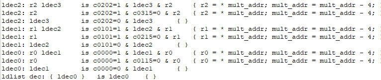
The example below describes only rangeDst, rangeDst1, and rangeDst2, so as not to clutter the article. This is sufficient to gain an understanding of the type of such tables; a full version is available in the project source files on github. In essence, when working with rangeDst, the chain of constructors will be processed in ascending order of the X index in rangeDstX until the start register is met. Then the chain of constructors that corresponds in length with the size of the range will be processed.
# «^» used to keep spaces from being cut off, view beginning of paper

# rangedstX: ...
# rangedstX: ...

rangeDst2: ^ r2 rangeDst3 is r2; rangeDst3; offStart = 0xf9 [counter = counter -1; offStart = offStart -1;] {}
rangeDst2: ^ a2 rangeDst3 is a2; rangeDst3; offStart = 0x04 [counter = counter -1; offStart = offStart +1;] {}
rangeDst2: } is epsilon; counter = 0; offStart = 0xf9 {}
rangeDst2: } is epsilon; counter = 0; offStart = 0x04 {}
rangeDst2: rangeDst3 is rangeDst3 {}
rangeDst1: ^ r1 rangeDst2 is r1; rangeDst2; offStart = 0xfa [counter = counter -1; offStart = offStart -1;] {}
rangeDst1: ^ a1 rangeDst2 is a1; rangeDst2; offStart = 0x03 [counter = counter -1; offStart = offStart +1;] {}
rangeDst1: } is epsilon; counter = 0; offStart = 0xfa {}
rangeDst1: } is epsilon; counter = 0; offStart = 0x03 {}
rangeDst1: rangeDst2 is rangeDst2 {}
rangeDst: ^ r0 rangeDst1 is r0; rangeDst1; offStart = 0xfb [counter = counter -1;offStart = offStart -1;] {}
rangeDst: ^ a0 rangeDst1 is a0; rangeDst1; offStart = 0x02 [counter = counter -1;offStart = offStart +1;] {}
rangeDst: } is epsilon; counter = 0; offStart = 0xfb {}
rangeDst: } is epsilon; counter = 0; offStart = 0x02 {}
rangeDst: rangeDst1 is rangeDst1 {}
Constructors with closing curly brackets look similar; you can try combining them. Remember to use the logical operators “&” and “|.”
# it is necessary for the sleigh compiler to use ‘( )’ here
rangeDst: } is epsilon; counter = 0; (offStart = 0xfb | offStart = 0x02) {}
The constructor for CallProperty in the completed project appears as follows:
define pcodeop CallVariadicCallOther;

# Call <callable> <receiver> <arg_count> <feedback_slot_id>
# Call a JSfunction or Callable in |callable| with the |receiver| and
# |arg_count| arguments in subsequent registers. Collect type feedback
# into |feedback_slot_id|

:CallProperty callable, rangeSrc^rangeDst, [kIdx] is op = 0x4a; callable; rangeSrc; rangeDst; kIdx {
# setting sizes for arguments of pcodeop functions as mentioned before
# in next paper you`ll see how you can turn this stub into crafted pcode instructions via java-code
	CallVariadicCallOther($(PROPERTYTYPE):4, $(RECV_ARG):4);
}
This is what we get in the listing:

It is perhaps confusing right now that the user-defined operation CallVariadicCallOther is used in the semantics actions section. In the project on github it was redefined in Java code using p-code instructions. The use of the p-code injection technique instead of the implementation via the call operation was the result of the desire to see the list of passed arguments in the decompiler (according to the Node.js source code, the first range register is the receiver, while the rest are the passed arguments). To put it mildly, it would be difficult to achieve this using only SLASPEC:
If you want to try to repeat the implementation of ranges yourself, you can describe the semantics as:
define pcodeop CallProperty;

# Call <callable> <receiver> <arg_count> <feedback_slot_id>
# Call a JSfunction or Callable in |callable| with the |receiver| and
# |arg_count| arguments in subsequent registers. Collect type feedback
# into |feedback_slot_id|

:CallProperty callable, rangeSrc^rangeDst, [kIdx] is op = 0x4a; callable; rangeSrc; rangeDst; kIdx {
	CallProperty(callable, rangeSrc, range_size);
}
Then, by analogy, we can extend the rangeDstХ constructors (we will need up to including r7 ) and then try to see what the compiled code of console.log(1,2,3,4,5,6) looks like. You can compile it yourself via bytenode or pick up the built one here. The function will be located at offset 0x167, while the instruction itself, at 0x18b.
In the end, instructions implying calls even with a constant number of arguments, were implemented in a similar fashion to resolve problems that arise during decompilation, as there was frequent confusion when counting the number of arguments because of the nuance with the initialization of the aX registers (it appears upon the launch of autoanalysis, it is sometimes encountered to date and is resolved, as in modules for other architectures, by changing the function prototype in the decompiler).
It is worth noting that in our project, we moved all the rangeDst constructors into a separate file so as not to clutter up the file with the description of instructions (as well as Wide and ExtraWide instructions that work with operands of 2 and 4 bytes):
@include 'ranges.sinc'Result
The developed processor module meets the requirements that we set for it: the tool makes it possible to view bytecode instructions for the specified functions of the file, which had to be parsed within the project. As a bonus, we got a decompiler, albeit not a perfect one, but still allowing you to navigate the application logic faster. However, as with many processor modules, in this case, it is better to view the instructions directly, rather than blindly trusting the decompiler. It can also be noted that, if given the time and desire to improve the tool, it would be worthwhile to implement type storage, devise an import concept, and eliminate the problem with the reverse order of function arguments. We hope this tutorial will make it easier for you to write processor modules in SLEIGH.
I would also like to extend my thanks to my colleagues Vyacheslav Moskvin, Vladimir Kononovich, and Sergey Fedonin with whom we researched Node.js and developed the module.
Helpful links
- ghidra.re/courses/languages/html/sleigh.html: documentation for SLEIGH
- github.com/NationalSecurityAgency/ghidra/tree/master/Ghidra/Framework/SoftwareModeling/data/languages: useful files with descriptions of .cspec, .pspec, .opinion, and *.ldefs
- spinsel.dev/2020/06/17/ghidra-brainfuck-processor-1.html: a decent article on implementing a brainfuck module in Ghidra
- github.com/PositiveTechnologies/ghidra_nodejs: a repository with a full version of the processor module for Ghidra with a loader and analyzer
P.S.
Several times the question about where to get descriptions of instructions in order to describe other versions of Node.js, etc. was asked. Here is our answer with some tips for getting started:
- The list of instructions is stored in the bytecodes.h file of Node.js. They are organized in ascending order by instruction code: Here you can also find the descriptions of operands. However, it will be quicker and easier to copy this list from a compiled binary file node.exe in function:
const char *__cdecl v8::internal::interpreter::Bytecodes::ToString(v8::internal::interpreter::Bytecode bytecode)- In interpreter-generator.cc you can take a look at the instruction semantics to understand what these instructions do.
- When writing instruction semantics, do not forget about registers that are not explicitly used in the instruction. For example, keep an eye on the accumulator to understand where it changes its value. Ghidra optimizes the decompiler output, and you can lose a part of the logic.
- Codes of instructions and operands take one byte (for regular instructions). As for
Wide-иExtraWide-instructions, the instruction code takes 2 bytes, and most of operand types take 2 or 4 bytes, respectively (operands withkFlag8do not grow in size). It will be easier to write code for regular instructions and then modify it for wider instructions. - It is actually quite easy to write a disassembler or a decompiler based on user-defined operations. You can start with listing output and a primitive decompiler and then add semantics and other details.
- Files bytecode-register.cc and bytecode-register.h will be useful to understand the registers index computation